Underwater Image Enhancement with Multiscale Feature Disentanglement

01 — Overview

Underwater photos are blue-green, hazy and low in contrast, because water absorbs and scatters light unevenly. I re-implemented MD-Net, a multiscale disentanglement network for underwater image enhancement (Yan et al., Scientific Reports, 2025), trained it on the LSUI and UIEB datasets, and evaluated it on three test sets with five metrics and five classical baselines.

What came out of it:

• The network lifts PSNR from 13.3 dB to 21.5 dB on LSUI and from 17.0 dB to 20.3 dB on UIEB, and it beats all five classical baselines on every full-reference metric (PSNR, SSIM, LPIPS) on both datasets.
• My absolute numbers do not match the paper’s. The paper does not say which images form its test sets, so mine are different, and harder. This page explains how I compared fairly anyway.
• Along the way I found and fixed an evaluation bug that made good outputs look broken, and documented the failure cases instead of hiding them.

02 — Problem

An underwater image is not simply a darker or lower-contrast version of a clear one. Water attenuates each wavelength differently, so red disappears within a few metres, and suspended particles scatter light back toward the camera as haze. The task is to recover a clear, naturally coloured image from a single degraded photo.

The paper uses the classic simplified imaging model:

I(x) = J(x) · t(x) + B · (1 − t(x))

where I is the observed image, J the clear scene radiance, t the transmission map and B the global background light.

03 — Why the problem is difficult

• It is ill-posed. Three unknowns (J, t, B) have to be estimated from one image.
• Degradation is not uniform. It depends on depth, water type, lighting and wavelength, so a single global colour or contrast correction does not work.
• There is no true ground truth. The reference images in UIEB were selected by human raters from the outputs of several enhancement methods, so “close to the reference” is only a proxy for “good”.
• Metrics disagree. Full-reference metrics (PSNR, SSIM, LPIPS) and no-reference ones (UCIQE, UIQM) can rank the same methods differently, because the no-reference metrics reward contrast.

04 — Approach

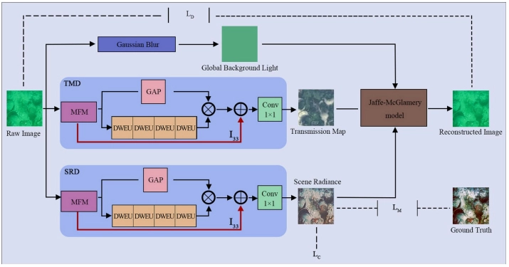
MD-Net does not map a degraded image straight to a clear one. It disentangles the image into the physical quantities of the imaging model, then checks itself by recombining them:

1. one sub-network estimates the clear image J,
2. a second, identically structured sub-network estimates the transmission map t,
3. a heavy Gaussian blur of the input provides the background light B,
4. the three are recombined into a reconstructed input I', and a loss compares I' with the real input.

This ties the network’s predictions to the physics of the problem instead of leaving it a black-box image-to-image model.

I followed the paper and the authors’ public implementation for the architecture. My contribution is the training pipeline, a careful evaluation, the baselines and the analysis of where it works and where it does not.

05 — Architecture

                  ┌────► SRD (scene radiance) ───────► J  enhanced image
input image I ────┼────► TMD (transmission map) ─────► t
                  └────► Gaussian blur ──────────────► B  background light
                                   │
                  I' = J·t + B·(1 − t)  ──►  compared with I (reconstruction loss)

SRD and TMD use the same architecture with separate weights. Each is built from two custom blocks:

• Multi-level fusion module (MFM). Three parallel branches with 3×3, 5×5 and 7×7 convolutions capture detail and context at different receptive fields. A small network predicts per-pixel weights that fuse the three branches.
• Dual-layer weight estimation unit (DWEU). A stack of four residual units, each combining channel attention (which feature maps matter) with pixel attention (which locations matter).

The blocks are separate, reusable PyTorch modules (custom_blocks/), assembled into the full network in neural_net.py.

06 — Mathematical formulation

The training loss has three terms, weighted equally:

L = L_A + L_C + L_M

L_A = MSE( I , I' )                      reconstruction: the recombined image should match the input
L_C = Σ_c ( mean(J_c) − 0.5 )²           gray-world colour prior on the enhanced image
L_M = MSE( J , reference )               supervised term against the reference image

L_A is what the paper calls a pseudo-adversarial loss: a feature-level reconstruction error rather than a full GAN. The paper does not state the weights of the three terms (its total-loss equation even contains a typo), so the 1:1:1 weighting is my assumption.

07 — Implementation

The repository is organised as reusable modules rather than one training notebook:

model/
  custom_blocks/   MFM, DWEU, pixel/channel weight layers, background light
  datasets/        paired dataset and the reference-free challenging set
  neural_net.py    SRD + TMD + imaging model
  total_loss.py    L_A + L_C + L_M
  trainer.py       training/validation loop with checkpoints and resume
  util.py          tensor ↔ image conversion (with clamping), checkpoint loading
uie_metrics.py     PSNR, SSIM, UCIQE, UIQM
colab_notebook.ipynb   training, testing, baselines, LPIPS, SIFT/Canny, figures

Three engineering lessons that mattered as much as the model:

• Clamp before saving. The network output is unbounded. Converting out-of-range values to 8-bit without clamping makes them wrap around, producing red dots and blown-out patches that looked like model failures. Clamping to [0, 1] fixed them.
• Verify the checkpoint is loaded. At one point I misread poor results as a generalisation problem, when the evaluation was actually running an untrained network. I added a sanity check that warns if the output statistics look untrained.
• Compare at the same resolution. UIQM and UCIQE depend on image size, so raw images are resized to the model’s input size before comparison.

08 — Experimental setup

Item	Setting
Training data	3,794 LSUI pairs + 800 UIEB pairs
Test data	485 LSUI, 90 UIEB, 60 UIEB Challenging (no reference)
Input size	350 × 350
Optimizer	Adam, learning rate 1e-4
Schedule	50 epochs, batch size 4
Metrics	PSNR, SSIM, LPIPS (full-reference); UCIQE, UIQM (no-reference)
Baselines	Gray-World, CLAHE, Gray-World + CLAHE, DCP, UDCP (my implementations, default parameters)
Downstream test	SIFT matches and Canny edge agreement against the reference

I used the paper’s split sizes, taking images in sorted file-name order, because the paper does not specify which images are in the test sets.

09 — Results

MD-Net against the raw input

Dataset	Method	PSNR ↑	SSIM ↑	LPIPS ↓	UCIQE ↑	UIQM ↑
LSUI	Raw	13.27	0.712	0.515	0.426	1.98
LSUI	MD-Net	21.53	0.895	0.204	0.558	2.66
UIEB	Raw	17.04	0.765	0.251	0.518	2.54
UIEB	MD-Net	20.33	0.872	0.167	0.596	2.89
Challenging	Raw	–	–	–	0.474	1.92
Challenging	MD-Net	–	–	–	0.560	2.33

Against classical methods (full-reference metrics; best in bold)

Method	LSUI PSNR	LSUI SSIM	LSUI LPIPS ↓	UIEB PSNR	UIEB SSIM	UIEB LPIPS ↓
Raw	13.27	0.712	0.515	17.04	0.765	0.251
Gray-World	14.94	0.765	0.329	16.72	0.771	0.306
CLAHE	13.87	0.782	0.439	17.09	0.799	0.239
Gray-World + CLAHE	15.91	0.828	0.265	17.09	0.801	0.282
DCP	13.02	0.678	0.430	15.34	0.729	0.246
UDCP	12.00	0.613	0.394	12.45	0.618	0.304
MD-Net	21.53	0.895	0.204	20.33	0.872	0.167

Two caveats worth reading:

• Contrast-driven metrics favour CLAHE. On the no-reference UIQM, Gray-World + CLAHE scores higher than MD-Net on UIEB (3.03 vs 2.89) and on the Challenging set (2.45 vs 2.33). UIQM rewards contrast and sharpness, which CLAHE raises directly, so I read it next to the full-reference metrics and the images.
• Supervised vs. training-free. MD-Net learns from the reference images and the classical methods do not, so full-reference metrics naturally favour it.

Downstream check. Canny edge agreement with the reference is highest for MD-Net on both datasets (F1 0.745 on LSUI, 0.862 on UIEB). SIFT matches with the reference are highest for MD-Net on LSUI (594 vs 507 for CLAHE), while CLAHE leads on UIEB (841 vs 803).

Against the paper.

Dataset	Paper (PSNR / SSIM)	This work (PSNR / SSIM)
LSUI	23.21 / 0.837	21.53 / 0.895
UIEB	24.05 / 0.892	20.33 / 0.872

I do not claim to match or beat the paper. My raw-input numbers differ from the paper’s too (for example 13.3 vs 21.3 dB PSNR on LSUI), which shows my test images are different and harder, so absolute values are not comparable. The improvement over raw is the fairer yardstick: +8.3 dB here vs +1.9 dB in the paper on LSUI, and +3.3 dB vs +4.9 dB on UIEB.

10 — Qualitative comparison

Each row is one test image; columns are raw input, CLAHE, Gray-World + CLAHE, MD-Net and the reference. Rows include good, median and the worst cases by PSNR, so the grid does not show only the best results.

My own visual impression, which is subjective (there was no user study): MD-Net corrects the blue-green cast more naturally than the baselines, and in many images its colours look more natural than the dataset reference itself. Gray-World + CLAHE and the references are often crisper.

11 — Failure cases

• Red-dominated images. When an image already has a red cast instead of the usual blue-green, the result is poor. My hypothesis, which I have not verified, is that the network learned to boost red because red is the most attenuated colour in the training data, so images that are already red-heavy get over-corrected.
• Residual haze. Some outputs keep a faint, diffuse whitish veil, and overall contrast is lower than CLAHE-based methods.
• Questionable references. Some of the lowest PSNR scores may come from the reference rather than the output: the paper itself points out colour distortion in some reference images of these datasets. I have not checked this image by image.

12 — What I learned

• Turning a paper into working software means resolving what it leaves unsaid: loss weights, normalisation choices and which images are in the test set. I had to decide, and document, each of them.
• Evaluation deserves as much engineering as the model. A one-line missing clamp and an unloaded checkpoint each produced convincing but wrong conclusions until I added checks for them.
• Metrics measure different things. Looking at five metrics, five baselines and the actual images gave a far more honest picture than any single number.
• Reproducing a result and explaining a result are different jobs. Comparing improvement over the raw input, rather than absolute numbers, was the only fair way to relate my results to the paper’s.

What I would improve next

• Fix the background-light computation inherited from the reference code, which uses only the first image of each batch, and retrain to see the effect.
• Run ablations (without the DWEU or the reconstruction loss) to check the paper’s claims.
• Measure the effect on a real downstream task, such as object detection accuracy on enhanced vs raw frames, and test on footage from a different camera and water type.

13 — Code / paper

• Code: github.com/BassamXYZ/md-net-underwater-image-enhancement (code, Colab notebook, result tables; pretrained weights in the Releases)
• Paper: J. Yan et al., Underwater image enhancement via multiscale disentanglement strategy, Scientific Reports 15, 6076 (2025). doi.org/10.1038/s41598-025-89109-7

This is an independent re-implementation for learning purposes and is not affiliated with the paper’s authors. Datasets: LSUI and UIEB, used under their own terms.